1. Introduction
Scaling Pandas DataFrame aggregations can be tricky. I learned that while solving a specific problem involving aggregates on group by expressions.
While it's certainly possible to squeeze out a lot of performance in Pandas in a single-threaded environment, the nature of Pandas makes it hard to scaleembarrassingly parallel problems. This frequently involves calculations on DataFrames where the individual results are dependent only on specific segments of a DataFrame, such as weeks or months. In this case, a DataFrame could be split apart into many DataFrame across segment boundaries and the calculations could theoretically be distributed across many threads, or even machines.
At the same time, Pandas already is a complex library with a lot of moving parts, so I can understand the decision to not build in parallelization. This is where Dask comes in handy. With Dask, users can parallelize computations on Pandas DataFrames. Not only does Dask parallelize computations on one machine, it also lets you scale them to run on more than one machine. It's also important to mention that Dask can run computations on DataFrames that are bigger than available RAM. It achieves this by only reading the parts into memory that are currently needed and immediately freeing up memory as soon as it doesn't need that data anymore. This can be especially handy when your computation needs a lot of intermediate steps.
This article covers two topics.
- How to create DataFrames in Pandas and Dask
- How to perform group by operations on Pandas and Dask DataFrames
First, we go through DataFrames creation in both Pandas and Dask. We use randomized weather data for our data analysis. After creating the data, I show how to calculate certain metrics and statistics using groupby().
2. Creating the DataFrames
First, we take a look at how to create data frames in Pandas and Dask.
2.1. Pandas
One way of creating DataFrames from pandas.Series objects is by creating a dictionary of the data and passing it to the pandas.DataFrame constructor, like so:
pd.DataFrame(
    {
        'column_a': pd.Series(...),
        'column_b': pd.Series(...),
    },
    index=pd.Series(...)
)
First, we load some libraries. We import dask.dataframe and pandas to create DataFrames and series in both libraries. We also import numpy for random data creation.
import pandas as pd
import dask.dataframe as dd
import numpy as np
np.random.seed(1)
We set the start date to 2001-01-01.
start = '2001-01-01'
The data we initialize consist of two columns and one index:
- Index: A date and timestamp combination starting in
2001-01-01ranging up to n and filled with one entry per day. - Rain: Indicates whether it rained on that day. Stored as a boolean. The value is true with a 50 % likelihood.
- Temperature: The temperature on that day. Uniformly selected from
[5, 30), a half-open interval.
def create_df(n_days):
    dates = pd.date_range(start, periods=n_days, freq='D', name='Date')
    rainy_days = np.random.choice([False, True], n_days)
    temperatures = np.random.randint(5, 30, n_days)
    # Combine Pandas Series into DataFrame
    return pd.DataFrame(
        {
            'Rain': rainy_days,
            'Temperature': temperatures,
        },
        index=dates,
    )
We create example data for 2 weeks.
create_df(14)
Output:
| Date | Rain | Temperature |
|---|---|---|
| 2001-01-01 | True | 18 |
| 2001-01-02 | True | 11 |
| 2001-01-03 | False | 23 |
| 2001-01-04 | False | 25 |
| 2001-01-05 | True | 10 |
| 2001-01-06 | True | 23 |
| 2001-01-07 | True | 25 |
| 2001-01-08 | True | 16 |
| 2001-01-09 | True | 15 |
| 2001-01-10 | False | 19 |
| 2001-01-11 | False | 23 |
| 2001-01-12 | True | 9 |
| 2001-01-13 | False | 28 |
| 2001-01-14 | True | 28 |
2.2. Dask
To create a Dask DataFrame, we use the existing Pandas DataFrame creation function and use Dask.dataframe.from_pandas to convert it into a chunked Dask DataFrame. As chunk size we use the amount of days in a year. The idea with chunk sizes is to use a big enough number as this dictates the size of an individual Pandas DataFrame.
Since Dask performs operations on individual Pandas DataFrames, it's important to choose a number that's useful for the kind of operation you want to perform on a DataFrame. To group by years, we tell Dask to use a chunk size of 365 days.
def create_ddf(n_days):
    df = create_df(n_days)
    return dd.from_pandas(df, chunksize=365)
We can see that Dask DataFrames don't immediately return a result. Rather, we have to compute it first:
create_ddf(7)
Output:
| npartitions=1 | Rain | Temperature |
|---|---|---|
| 2001-01-01 |
bool
|
int64
|
| 2001-01-07 | … | … |
A Dask DataFrame can be evaluated by calling the compute() method on it. Since we are not using Dask.distributed right now, Dask runs the calculation in on one thread.
create_ddf(7).compute()
Output:
| Date | Rain | Temperature |
|---|---|---|
| 2001-01-01 | False | 13 |
| 2001-01-02 | False | 12 |
| 2001-01-03 | True | 8 |
| 2001-01-04 | True | 11 |
| 2001-01-05 | True | 26 |
| 2001-01-06 | False | 22 |
| 2001-01-07 | True | 8 |
3. Longest number of consecutive rainy days
3.1. Algorithm
For our first group by, we would like to find the longest chain of rainy days in the whole DataFrame. We use a neat trick for this. Using a combination ofSeries.shift() and Series.cumsum(), we can create an auxiliary series that tracks the difference and lets us perform a group by on the difference list.
Let's take a look at an example. First, a DataFrame is created with 2 consecutive rainy days
sunny_example = pd.DataFrame(
    {
        'Rain': [False, False, False, True, True, False],
        'Date': [0, 1, 2, 3, 4, 5],
    }
)
sunny_example
Output:
| Date | Rain | |
|---|---|---|
| 0 | 0 | False |
| 1 | 1 | False |
| 2 | 2 | False |
| 3 | 3 | True |
| 4 | 4 | True |
| 5 | 5 | False |
Using Series.shift() a difference list is calculated.
diff = sunny_example.Rain != sunny_example.Rain.shift()
diff.to_frame()
Output:
| Rain | |
|---|---|
| 0 | True |
| 1 | False |
| 2 | False |
| 3 | True |
| 4 | False |
| 5 | True |
Now, the value is True only when the weather changes from rainy to sunny or vice versa. Following this, the difference list is summed up usingSeries.cumsum().
diff.cumsum().to_frame()
Output:
| Rain | |
|---|---|
| 0 | 1 |
| 1 | 1 |
| 2 | 1 |
| 3 | 2 |
| 4 | 2 |
| 5 | 3 |
You can group rainy and non-rainy consecutive days using these values:
sunny_example_result = sunny_example.groupby(diff.cumsum()).Rain.agg(
    ['min', 'max', 'count'],
)
sunny_example_result
Output:
| Rain | min | max | count |
|---|---|---|---|
| 1 | False | False | 3 |
| 2 | True | True | 2 |
| 3 | False | False | 1 |
And the longest series of rainy days can be retrieved. min and max beingTrue tells us that the days in question only contain the boolean value Trueand because of that are rainy days.
query_result = sunny_example_result.query('min == max == True')['count']
max_idx = query_result.idxmax()
print(max_idx)
sunny_example_result.loc[max_idx].to_frame()
Output:
2
Output:
| 2 | |
|---|---|
| min | True |
| max | True |
| count | 2 |
3.2. Pandas
First, we define the number of days for the example calculation with the following snippet:
years = 100
days = years * 365

aggregate = [
    'min', 'max', 'count',
]
Using the steps outlined before, the function operating on Pandas DataFrames is defined.
def df_consecutive(df):
    df = df.reset_index()
    # Create difference list
    diff = (df.Rain != df.Rain.shift()).cumsum()
    # Aggregate longest consecutive occurences
    agg = df.groupby(diff).Rain.agg(aggregate)
    # Return length of longest consecutive occurence
    return agg.query('min == max == True')['count'].max()
Let's verify the result by running our function on the previous example DataFrame.
df_consecutive(sunny_example)
Output:
2
And we see that everything works as it's supposed to. Lastly, we time the execution using the %%timeit IPython magic command.
%%timeit
df_consecutive(create_df(days))
Output:
21.5 ms ± 1.06 ms per loop (mean ± std. dev. of 7 runs, 10 loops each)
3.3. Dask
Dask can take any algorithm that we've developed using Pandas and turns it into a Dask compatible execution graph. As the code below demonstrates, in simple cases we do not have to adjust anything at all and can just go on using our existing Pandas code.
def ddf_consecutive(ddf):
    ddf = ddf.reset_index()
    # Create difference list
    diff = (ddf.Rain != ddf.Rain.shift()).cumsum()
    # Aggregate longest consecutive occurences
    agg = ddf.groupby(diff).Rain.agg(aggregate)
    # Return length of longest consecutive occurence
    return agg.query('min == max == True')['count'].max()
As an intermediate step, the previous example DataFrame is turned into a Dask DataFrame.
sunny_example_Dask = dd.from_pandas(sunny_example, chunksize=365)
sunny_example_Dask
Output:
| npartitions=1 | Date | Rain |
|---|---|---|
| 0 |
int64
|
bool
|
| 5 | … | … |
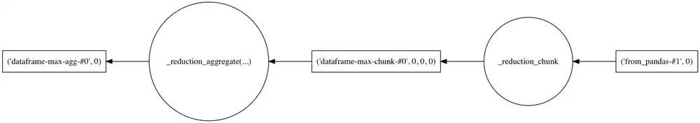
The computation graph for creating a Dask DataFrame from Pandas and retrieving the highest value can be visualized with ease.
sunny_example_Dask.max().visualize(optimize_graph=True, layout='circo')
Output:
Using the same Dask function we have specified before, we verify one more time that the result is calculated correctly.
b = ddf_consecutive(sunny_example_Dask)
b.compute()
Output:
2
The function is timed using the IPython %%timeit command. The Dask example is at least 10 times slower.
%%timeit
ddf_consecutive(create_ddf(days)).compute()
Output:
2.49 s ± 97.8 ms per loop (mean ± std. dev. of 7 runs, 1 loop each)
4. Determine the coldest weeks
For the second example, the coldest week in a DataFrame is determined.
4.1. Algorithm
To retrieve the coldest week, a combination of resampling and indexing is used. We create an example DataFrame:
cold_example = pd.DataFrame(
    {
        'Temperature': [0, 0, 0, 0, 0, 0, 0, 1, 1, 1, 1, 1, 1, 1]
    }, index=pd.date_range(start='2017-01-01', periods=14)
)
cold_example
Output:
| Temperature | |
|---|---|
| 2017-01-01 | 0 |
| 2017-01-02 | 0 |
| 2017-01-03 | 0 |
| 2017-01-04 | 0 |
| 2017-01-05 | 0 |
| 2017-01-06 | 0 |
| 2017-01-07 | 0 |
| 2017-01-08 | 1 |
| 2017-01-09 | 1 |
| 2017-01-10 | 1 |
| 2017-01-11 | 1 |
| 2017-01-12 | 1 |
| 2017-01-13 | 1 |
| 2017-01-14 | 1 |
To resample the temperature by weeks, we can use the DataFrame.resample()method. We take extra care to resample only full weeks and only those that fully start in the year 2017.
grouper = cold_example.Temperature.resample('W-MON', label='left')
grouper
Output:
DatetimeIndexResampler [freq=<Week: weekday=0>, axis=0, closed=right, label=left, convention=start, base=0]
For our purposes, the semantics of a Dask resample() and Pandas grouper are the same. We can apply aggregate() functions such as sum() and count(). In this case, count() tells us the length of a grouped week and the sum of the daily temperatures.
It becomes evident below that there are two partial weeks in the dataset. One begins in the last year, and the other week doesn't have enough days in the current year. Because of that, the only usable week is the one starting in2017-01-02.
agg = grouper.aggregate(['sum', 'count'])
agg
Output:
| sum | count | |
|---|---|---|
| 2016-12-26 | 0 | 2 |
| 2017-01-02 | 2 | 7 |
| 2017-01-09 | 5 | 5 |
We can then filter out partial weeks with the following query:
agg.query("count == 7")
Output:
| sum | count | |
|---|---|---|
| 2017-01-02 | 2 | 7 |
And the coldest week is the following:
agg.query("count == 7")['sum'].idxmin()
Output:
Timestamp('2017-01-02 00:00:00', freq='W-MON')
4.2. Pandas
For Pandas, we create a single function to find the coldest week:
def df_coldest_week(df):
    weeks = df.Temperature.resample(
        'W-MON',
        label='left',
    ).agg(['count', 'sum']).query('count == 7')
    return weeks['sum'].idxmin()
We can verify that the result is correct.
df_coldest_week(cold_example)
Output:
Timestamp('2017-01-02 00:00:00', freq='W-MON')
A quick %%timeit is run on the Pandas function.
%%timeit
df_coldest_week(create_df(days))
Output:
151 ms ± 3.53 ms per loop (mean ± std. dev. of 7 runs, 10 loops each)
4.3. Dask
Since Dask resample() does not support aggregates at the time of writing, we have to trick around a little bit to get it to work.
def ddf_coldest_week(df):
    weeks = df.Temperature.resample(
        'W-MON',
        label='left',
    )
    # Calculate week lengths
    count = weeks.count()
    # Sum temperatures
    sum = weeks.sum()
    # Select results by week day lengths.
    loc = count == 7
    return sum[loc].idxmin()
We run the function on our example DataFrame. First, we turn it into a Dask DataFrame.
cold_example_Dask = dd.from_pandas(cold_example, npartitions=1)
As we can see, the computed result is exactly the same.
ddf_coldest_week(cold_example_Dask).compute()
Output:
Timestamp('2017-01-02 00:00:00')
Now we run the benchmark and discover that the Dask example takes about 10 times longer to execute.
%%timeit
ddf_coldest_week(create_ddf(days)).compute()
Output:
2.45 s ± 26.5 ms per loop (mean ± std. dev. of 7 runs, 1 loop each)
5. Benchmarks
The benchmark results show that using Dask performs slower on the small datasets that we have created. Whether this applies to bigger sized datasets as well was not established in this article. What stands true in any case is that Dask can work with datasets that are larger than the available memory, and are especially larger than any piece of continuously available memory in the OS. This lets you scale calculations while using almost the same code to data sets in the 500 GB to 1 TB range.
I was able to successfully apply these insights for a large amount of non-trivial A/B test calculations on user click data without having to set up a complicated computing cluster.
Taking the weather calculations that we've performed as an example, one can start by developing the aggregation functions using Pandas or Dask on a small data set and test it. Using the same function with minimal adjustments, the process can then be scaled to data sets with hundreds of measurement locations and still get reasonable performance across a multi-core machine or even a cluster. You can do this on an Amazon Web Services EC2 instance. The Dask documentationhas a tutorial on how to do this..
6. Further reading
The official Dask documentation is helpful when trying to figure out how to translate Pandas calculations to distributed Dask calculations. It is also always worth taking a look at Pandas tutorials when figuring out how to efficiently vectorize calculations.