The Pandas API surprises me with a new feature or method almost every day, and I've again discovered an interesting feature.
1. Introduction
Using .transform(), you can, excuse the pun, transform the way you aggregate
DataFrames. While not applicable to every use case in the
"split apply combine" workflow,
it makes one common task easy: joining back aggregate values to the original
DataFrame.
First, we create an example DataFrame to explore the many ways we can use
.transform() in our Data Analysis work flow.
We import Pandas for DataFrame creation, random for generation of random data
in our DataFrame, and datetime.datetime and datetime.timedelta for purchase
date creation. We furthermore import Matplotlib to inspect the data.
import pandas as pd
import random
from datetime import datetime, timedelta

import matplotlib.pyplot as plt
Just while creating this notebook I was struggling with one thing in particular
while playing around with DataFrame creation. DataFrames printed inside IPython
are sometimes just too long and have too many rows. Just typing df and having
a well-formatted HTML table of the head and tail of the DataFrame you want
to inspect come out is just too convenient.
I wondered whether there was any way to shorten the number of rows
printed when evaluating a DataFrame. pandas.set_option to the rescue. The
documentation has a full list of all options available, and one option
that we find interesting in particular is max_rows. It determines how many
rows Pandas can print at most when outputting truncated DataFrames.
Pandas truncates DataFrame outputs based on how much space is available for printing it. In the terminal, this is pretty easy to find out. Pandas just needs to see what the terminal's character dimensions are. With IPython and Jupyter, this is not so easy. There's no API available for determining the browser window dimensions inside Pandas. Thus, we're stuck with manually setting a value.
We choose 6 as the most rows to be shown, including the head and tail of a DataFrame.
pd.set_option('display.max_rows', 6)
Today's DataFrame, filled with fake data, consists of the following data.
Since we want to keep it entertaining, the data we look at today is e-commerce purchase data. We look at a table containing purchase items, and data that is associated with them. The purchase items are linked to a specific order ID. One purchase can contain more than one purchase item. To sum it up, we create the following columns.
date: Date of purchasecategory: Category of item, either Food, Beverage or Magazinevalue: Purchase value of item, ranges from 10 to 100customer: ID of customer that purchased this item, a random ID from 1 to 10purchase: ID of purchase, there are 30 purchases with IDs ranging from 1 to 30
random.seed(1)
category_names = [
    "Food",
    "Beverage",
    "Magazine",
]
start_date = datetime(2017, 1, 1)
rows = 100
df = pd.DataFrame(
    [
        [
            start_date + timedelta(
                days=random.randint(0, 30)
            ),
            random.choice(category_names),
            random.randint(10, 100),
            random.randint(1, 10),
            random.randint(1, 30),
        ]
        for _ in range(rows)
    ],
    columns=[
        "date",
        "category",
        "value",
        "customer",
        "purchase",
    ],
)
df.index.name = "item_id"
df
Output:
item_id |
date |
category |
value |
customer |
purchase |
|---|---|---|---|---|---|
| 0 | 2017-01-05 | Magazine | 18 | 5 | 4 |
| 1 | 2017-01-16 | Beverage | 70 | 7 | 26 |
| 2 | 2017-01-07 | Food | 72 | 1 | 29 |
| … | … | … | … | … | … |
| 97 | 2017-01-30 | Beverage | 41 | 6 | 4 |
| 98 | 2017-01-18 | Magazine | 84 | 10 | 3 |
| 99 | 2017-01-08 | Food | 12 | 4 | 13 |
That should give us some useful purchase data to work with.
2. The problem
The other day I was working on an interesting problem that I could only solve in a cumbersome way with Pandas before. For each purchase in a similar DataFrame, I wanted to calculate a purchase item's total contribution to the total purchase value. For example, if a customer bought two 10 US Dollar items for a total value of 20 US Dollars, one purchase item would contribute 50 % to the total purchase value.
To find the total purchase value, we would typically use a group by together
with a .sum(). Since we need to calculate the ratio of a purchase item's
value to the total purchase value, we would need to join that data back to the
original DataFrame. Or at least, this is how I would have done it before
finding out about .transform().
Let's take it step by step and look at the necessary calculation steps. First,
we need to group by a purchase ID and sum up the total purchase value. We need
to group by purchase and sum up the value column:
values = df.groupby('purchase').value.sum()
values.to_frame()
Output:
| purchase | value |
|---|---|
| 2 | 146 |
| 3 | 398 |
| 4 | 377 |
| … | … |
| 28 | 89 |
| 29 | 329 |
| 30 | 63 |
What we get is a Pandas Series containing the total purchase values for every
purchase ID. Since we used a group by on the purchase ID, purchase is the
index of this Series. We can visualize this data with a bar plot.
fig, ax = plt.subplots(1, figsize=(20, 5))
values.plot(kind='bar', ax=ax)
fig
Output:
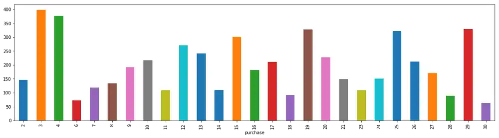
Bar chart showing the total purchase value for every purchase ID Open in new tab (full image size 6 KiB)
Now that we have the total purchase value for each purchase ID, we can join
this data back to the purchase DataFrame. For this, we perform a left join of
the purchase values to the DataFrame on purchase. We further specify that the
value of the right side should receive the suffix _total. If we take a look
again at our total purchase values, we can see that the name of the Series is
the following.
values.name
Output:
'value'
If you perform a join() without giving Pandas a suffix, it complains about a
name collision. This is because both sides specify a column named value,
which can not be joined, since it's unclear which column should take
precedence. We need to have the right side column in the Series that we are
joining change its name by using the suffix _total. Indicating that it's a
total value in the name of course makes a lot of sense, since the column
contains the total purchase values.
Let's perform the actual join then 🚀
df.join(values, on='purchase', rsuffix='_total')
Output:
item_id |
date |
category |
value |
customer |
purchase |
value_total |
|---|---|---|---|---|---|---|
| 0 | 2017-01-05 | Magazine | 18 | 5 | 4 | 377 |
| 1 | 2017-01-16 | Beverage | 70 | 7 | 26 | 213 |
| 2 | 2017-01-07 | Food | 72 | 1 | 29 | 329 |
| … | … | … | … | … | … | … |
| 97 | 2017-01-30 | Beverage | 41 | 6 | 4 | 377 |
| 98 | 2017-01-18 | Magazine | 84 | 10 | 3 | 398 |
| 99 | 2017-01-08 | Food | 12 | 4 | 13 | 241 |
As we have discussed before, we want to calculate the ratio of a single
purchase item to the total purchase value. We calculate
value / value_total * 100 to get the ratio as a percentage.
df.assign(
    value_pct=(
        df.value /
        df.join(
            values,
            on='purchase',
            rsuffix='_total',
        ).value_total *
        100
    )
).round(2)
Output:
item_id |
date |
category |
value |
customer |
purchase |
value_pct |
|---|---|---|---|---|---|---|
| 0 | 2017-01-05 | Magazine | 18 | 5 | 4 | 4.77 |
| 1 | 2017-01-16 | Beverage | 70 | 7 | 26 | 32.86 |
| 2 | 2017-01-07 | Food | 72 | 1 | 29 | 21.88 |
| … | … | … | … | … | … | … |
| 97 | 2017-01-30 | Beverage | 41 | 6 | 4 | 10.88 |
| 98 | 2017-01-18 | Magazine | 84 | 10 | 3 | 21.11 |
| 99 | 2017-01-08 | Food | 12 | 4 | 13 | 4.98 |
To be honest, for a long time I thought that this was the only way to do it. At the same time I was more than concerned with how burdensome joining values back to the original DataFrame is.
Browsing through the Pandas documentation led me to discover a useful method,
the .transform(). Time after time, aimlessly wandering through documentation
has brought positive change into my humble life.
Using transform, we simplify this process and make the present an even more exciting time to be alive in.
3. Transform to the Rescue
While .transform()'s API is well documented, I could only find a few hints to
what the use cases might be
in the documentation.
Now I would like to present the perfect use case for .transform(). First,
let's take a look at what the method exactly returns. We define a method that
prints the value it receives and returns the same value.
def return_print(value):
    print(value)
    return value
We then use .transform() to apply this function on our DataFrame. To avoid
the result from getting too long we only apply it to the category and value
column. We see that the category column is evaluated twice, which seems
strange. Read on to find out why.
df[['category', 'value']].transform(return_print)
Output:
item_id
0     Magazine
1     Beverage
2         Food
        ...
97    Beverage
98    Magazine
99        Food
Name: category, Length: 100, dtype: object
item_id
0     Magazine
1     Beverage
2         Food
        ...
97    Beverage
98    Magazine
99        Food
Name: category, Length: 100, dtype: object
item_id
0     18
1     70
2     72
      ..
97    41
98    84
99    12
Name: value, Length: 100, dtype: int64
Output:
item_id |
category |
value |
|---|---|---|
| 0 | Magazine | 18 |
| 1 | Beverage | 70 |
| 2 | Food | 72 |
| … | … | … |
| 97 | Beverage | 41 |
| 98 | Magazine | 84 |
| 99 | Food | 12 |
It's interesting to see that Pandas executes return_print on the first column
twice. That's why the same output Name: category, Length: 100, dtype: object
appears twice. To speed up execution, Pandas needs to find out which code path
it can execute, as there is a fast and slow way of transforming ndarrays.
Thus, the first column is evaluated twice. As always,
the documentation
describes this mechanism well (look for the Warning section).
We can furthermore observe that the result is an unchanged DataFrame. This is reassuring and lets us understand the next example even better.
We would like to calculate the standard score for each value. The standard score of a value is defined as
where
- is the standard deviation of all values, and
- is the mean of all values.
We can express this as a .transform() call, by calculating the following:
x - x.mean() / x.std()
x here denotes the column we are calculating the standard scores for. Since
not every column is numerical, we limit ourselves to the value column and
calculate standard scores for all purchase item values.
df.value.transform(
    lambda x: (x - x.mean()) / x.std()
).to_frame('value_standard_score')
Output:
item_id |
value_standard_score |
|---|---|
| 0 | -1.354992 |
| 1 | 0.643862 |
| 2 | 0.720741 |
| … | … |
| 97 | -0.470884 |
| 98 | 1.182015 |
| 99 | -1.585630 |
An observant reader notices that we can also perform the following calculation to retrieve the same result:
(
    (df.value - df.value.mean()) /
    df.value.std()
).to_frame('value_standard_score_alt')
Output:
item_id |
value_standard_score_alt |
|---|---|
| 0 | -1.354992 |
| 1 | 0.643862 |
| 2 | 0.720741 |
| … | … |
| 97 | -0.470884 |
| 98 | 1.182015 |
| 99 | -1.585630 |
That is correct. I can see both forms having their advantages and
disadvantages. I see the advantage of using .transform() instead of operating
on raw columns as the following:
- Define reusable methods, for example for standard score calculation, that can be applied over any DataFrame. Code reuse for the win.
- Avoid retyping the column name that you operate on. This means typing
xversus typingdf.valueall the time. .transform()can apply more than one transformation at once.
Let's take a look at an example for two transformations applied at the same time.
def standard_score(series):
    """Return standard score of Series."""
    return (series - series.mean()) / series.std()

def larger_median(series):
    """Return True for values larger than median in Series."""
    return series > series.median()

df.transform({
    'value': [
        standard_score,
        larger_median,
    ],
    'date': lambda ts: ts.day
})
Output:
value |
date |
||
|---|---|---|---|
standard_score |
larger_median |
lambda |
|
item_id |
|||
| 0 | -1.354992 | False |
5 |
| 1 | 0.643862 | True |
16 |
| 2 | 0.720741 | True |
7 |
| … | … | … | … |
| 97 | -0.470884 | False |
30 |
| 98 | 1.182015 | True |
18 |
| 99 | -1.585630 | False |
8 |
While we have observed in a
previous article that it's possible
to assign names to function calls in .aggregate() to give result columns new
names, it does not appear to be possible with transform.
For example, we were able to do the following with a tuple:
df.aggregate({
    'value': [
        ('mean', lambda x: x.sum() - x.count()),
    ],
})
We were then able to retrieve a column named mean that contains the result of
the lambda, but we can't do the same using .transform(). The
following is impossible:
df.value.transform({
    'value': [
        ('standard_score', lambda x: (x - x.mean()) / x.std()),
    ],
})
We would instead just be greeted by an irritated Exception telling us to reflect on our deeds.
Leaving that aside, I would like to show you another use case for .transform()
in the next section.
4. The problem, solved
It turns out that you can use .transform() in group by objects. What do
we do with that? We can now calculate the aggregate value, just like when
using .aggregate(), and then join it back to the index of the original
grouped by object. If we're calculating a sum for every group, we then add
the result back to each index that corresponds to that group.
When grouping by purchase and calculating a sum, we would be then adding the sum back to every purchase item. Then, we can look at one purchase item and know both the purchase item's value and the total purchase value.
Let's try it out then:
ts = df.groupby('purchase').value.transform('sum')
ts.to_frame()
Output:
item_id |
value |
|---|---|
| 0 | 377 |
| 1 | 213 |
| 2 | 329 |
| … | … |
| 97 | 377 |
| 98 | 398 |
| 99 | 241 |
Instead of directly calling .transform() on our well-known and beloved
DataFrame, we first group by the purchase ID column. Since there are
approximately 30 purchases, this creates approximately 30 groups.
Then, for each group we calculate the sum in the .transform('sum') call and
directly join that value back to the index used before the .groupby() call.
We can now join that value back to our original DataFrame:
df.join(ts, rsuffix='_total')
Output:
item_id |
date |
category |
value |
customer |
purchase |
value_total |
|---|---|---|---|---|---|---|
| 0 | 2017-01-05 | Magazine | 18 | 5 | 4 | 377 |
| 1 | 2017-01-16 | Beverage | 70 | 7 | 26 | 213 |
| 2 | 2017-01-07 | Food | 72 | 1 | 29 | 329 |
| … | … | … | … | … | … | … |
| 97 | 2017-01-30 | Beverage | 41 | 6 | 4 | 377 |
| 98 | 2017-01-18 | Magazine | 84 | 10 | 3 | 398 |
| 99 | 2017-01-08 | Food | 12 | 4 | 13 | 241 |
Even more exciting, we can perform the same calculation that we've performed
before, and achieve what required an extra .join() before.
df.assign(
    value_pct=(
        df.value /
        ts *
        100
    )
).round(2)
Output:
item_id |
date |
category |
value |
customer |
purchase |
value_pct |
|---|---|---|---|---|---|---|
| 0 | 2017-01-05 | Magazine | 18 | 5 | 4 | 4.77 |
| 1 | 2017-01-16 | Beverage | 70 | 7 | 26 | 32.86 |
| 2 | 2017-01-07 | Food | 72 | 1 | 29 | 21.88 |
| … | … | … | … | … | … | … |
| 97 | 2017-01-30 | Beverage | 41 | 6 | 4 | 10.88 |
| 98 | 2017-01-18 | Magazine | 84 | 10 | 3 | 21.11 |
| 99 | 2017-01-08 | Food | 12 | 4 | 13 | 4.98 |
In the end, we were able to avoid one unpleasant .join() call and have made
the intent behind our summation a lot clearer. And if you want to improve the
comprehensibility of your IPython notebooks, clear intent, terseness and
readability are king.
5. Summary
With .transform() in our toolbox, we've acquired yet another useful tool for
Data Analysis. It's always a delight to dig in the Pandas documentation to find
out what other delights this great library has to offer. I hope to be able to
write even more articles about obscure niches in the Pandas API and surprise
you with one or two things that neither of us knew about.
I would like to encourage you to stay tuned and go out, dig up some new Pandas DataFrame methods, and enjoy working with data.